Basic MCMC Usage

library(StructCoalescent)

Example

This is a basic example of usage. First, we sample a heterochronous dated structured phylogenetic tree with $n=10$ leaves obtained from from $d=3$ demes between 2015 and 2020.

n <- 10
d <- 3
leaf_data <- cbind('Leaf_ID'=paste0('L', 1:n),
                   'Leaf_age'=sample(2018:2020, n, TRUE),
                   'Leaf_deme'=sample(1:d, n, TRUE))
coalescent_rates <- rexp(d, 1)
migration_matrix <- matrix(rexp(d^2, 20), d, d); diag(migration_matrix) <- 0


strphylo <- rstrphylo(n, d, coalescent_rates, migration_matrix, leaf_data)
plot(strphylo, time_axis=TRUE, root_time=strphylo$root.age, show.tip.label=TRUE)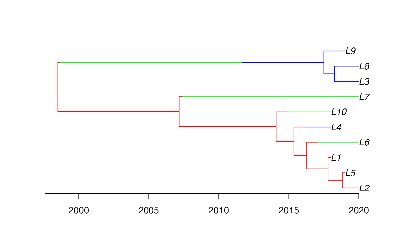

Our simulated phylogeny is returned as an object of class strphylo which can be passed directly into our MCMC algorithm as an initialisation point. Alternatively, we illustrate how to convert between a strphylo phylogeny and a BEAST-annotated Newick string using the treeio package.

A strphylo phylogeny can be converted to a Newick string via a treedata object as follows,

treedata <- treeio::as.treedata( strphylo )
newick_string <- treeio::write.beast.newick( treedata )

resulting in a Newick string

#> (((((((L2[&type=1]:1.173559841,L5[&type=1]:0.173559841)[&type=1]:1.018941774,L1[&type=1]:0.1925016146)[&type=1]:1.551420165,(L6[&type=2]:2.888916888)[&type=1]:0.8550048914)[&type=1]:0.8860324419,(L4[&type=3]:1.910819747)[&type=1]:0.7191344737)[&type=1]:1.270947111,(L10[&type=2]:3.106935748)[&type=1]:0.7939655846)[&type=1]:6.925557613,(L7[&type=2]:12.59366215)[&type=1]:0.2327967944)[&type=1]:8.663322076,((((L3[&type=3]:1.738566852,L8[&type=3]:1.738566852)[&type=3]:0.7562937879,L9[&type=3]:1.49486064)[&type=3]:5.827259607)[&type=2]:13.02874437)[&type=1]:0.1389164082)[&type=1];

We can then return from the annotated Newick string (with demes annotated by type) to our original strphylo object as follows

treedata <- treeio::read.beast.newick(
  textConnection( newick_string )
)
strphylo <- as.strphylo( treedata )

Note that we require textConnection() here to allow our Newick string (stored as a character vector) to be passed as a file connection into read.beast.newick(). Alternatively, a Newick string can be passed in from an external file using the path to the file.

Now that we have a structured phylogeny in strphylo format to use for initialisation, we identify the prior parameters for use in our MCMC. To use our default prior distributions, we can either omit all prior parameters from our MCMC,

# NOT RUN
StructCoalescent_mcmc(N=1e4, strphylo, coalescent_rates, migration_matrix, stdout_log=FALSE, thin=100, proposal_rates=c(20, 1, 1))

or we can pass prior parameters into the MCMC using in a mode-variance parameterisation of a Gamma distribution

prior_parameters <- default_priors( strphylo, n_deme = 3, M = fitch( strphylo )$min_migs )

#>     cr_shape      cr_rate      cr_mode       cr_var     mm_shape      mm_rate 
#> 1.000000e+00 3.745767e+00 0.000000e+00 7.127194e-02 1.000000e+00 4.645352e+01 
#>      mm_mode       mm_var 
#> 0.000000e+00 4.634071e-04

# NOT RUN
StructCoalescent_mcmc(N=1e4, strphylo, coalescent_rates, migration_matrix,
                      cr_mode = 0, cr_var = 0.443212770,
                      mm_mode = 0, mm_var = 0.001004854,
                      stdout_log=FALSE, thin=100, proposal_rates=c(20, 1, 1))

MCMC output consists of three files (by default added to current working directory getwd()):

• StructCoalescent.trees contains a thinned MCMC sample of dated structured phylogenies in a BEAST meta-commented Newick format, which can be read with treeio::read.beast.
• StructCoalescent.log contains a thinned MCMC sample of evolutionary parameters, likelihood evaluations and the current radius of the subtree in a csv format, which can be read with read.csv
• StructCoalescent.freq contains details of the total number of accepted proposals of each type as well as the total number of attempted proposals of that type.

We can present a sample of migration histories using a consensus migration history, with sections of the branch assigned a deme provided a proportion $p$ of sampled migration histories observe the same deme at that position as follows:

strphylo_list <- lapply(treeio::read.beast('./StructCoalescent.trees'), as.strphylo)
consensus_strphylo <- exact_consensus(strphylo_list, consensus_prob=0.75)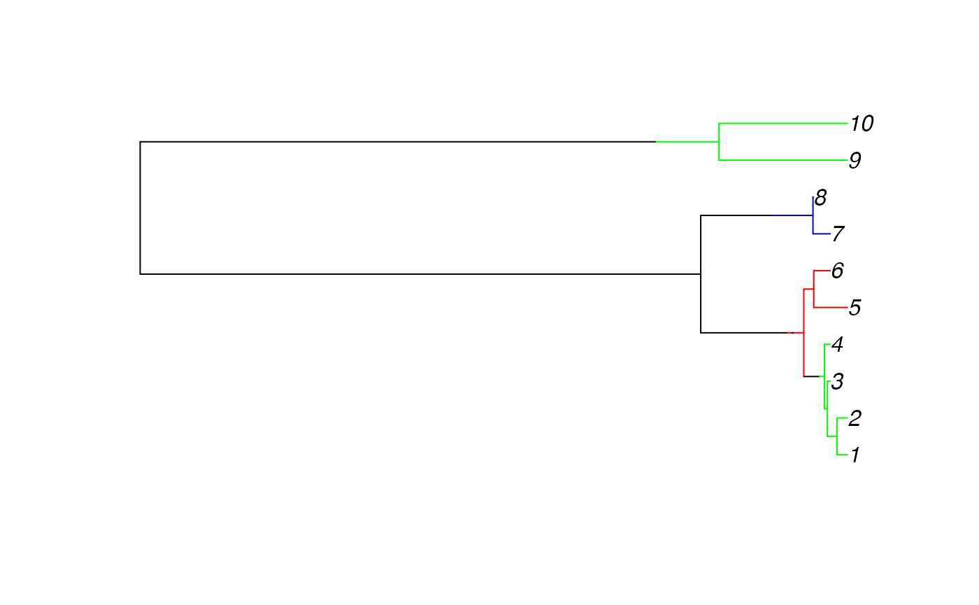

Evolutionary parameter samples can be presented in a variety of ways including trace plots and histograms:

Trace plots

StructCoalescent_log <- read.csv('./StructCoalescent.log',
                                 header=TRUE)
# layout(matrix(1:d^2, d, d))
for (col_id in 1:d){
  for (row_id in 1:d){
    if (col_id == row_id){
      col_name <- paste0('coal_rate_', col_id)
      title <- list(paste0('theta[', col_id, ']'))
      true_param <- coalescent_rates[col_id]
    } else{
      col_name <- paste('backward_migration_rate', row_id, col_id, sep='_')
      title <- paste0('lambda[', row_id, ',', col_id, ']')
      true_param <- migration_matrix[row_id, col_id]
    }
    plot(StructCoalescent_log$sample, StructCoalescent_log[,col_name], type='l', xlab='Sample', ylab=title)
    abline(h=true_param, lty=2, col='red')
  }
}

Histograms

StructCoalescent_log <- read.csv('./StructCoalescent.log',
                                 header=TRUE)
layout(matrix(1:d^2, d, d))
for (col_id in 1:d){
  for (row_id in 1:d){
    if (col_id == row_id){
      col_name <- paste0('coal_rate_', col_id)
      title <- list(paste0('theta[', col_id, ']'))
      true_param <- coalescent_rates[col_id]
    } else{
      col_name <- paste('backward_migration_rate', row_id, col_id, sep='_')
      title <- paste0('lambda[', row_id, ',', col_id, ']')
      true_param <- migration_matrix[row_id, col_id]
    }
    hist(StructCoalescent_log[,col_name], xlab=title, freq=FALSE, main='')
    abline(v=true_param, lty=2, col='red')
  }
}